For documentation on the current version, please check Knowledge Base.
Orbit Core Desktop Tutorial
All Orbit products are running on the same GIS Core, a platform based on Java technology. Although each Orbit product is designed to accomplish different parts in the general workflow, and have different functionalities and tools, they are all based on this core.
So this tutorial will guide you to the steps necessary to understand the basics of orbit products in order to be able to use afterwards the specific Orbit products. It’s just a tutotrial, all detailed explanation of each tool it is necessary to read the information on the Knowledge Database: tutorials
Software:
Orbit MM Content Manager 11.2.3 or
Orbit MM Feature Extraction
Software homepage:
Orbit Mobile Mapping Content Manager
Data : Generic , Gent, Belgium. Input data: Panoramic images (jpg), photo positions (csv), lidar data (las), ground control points (txt), reference data. Please copy the demo data provided to : D:\training\GENT
Necessary knowledge: Before starting working with the Orbit it is advised to first understand how Orbit sees MM data and what kind of data can be used. For this please read:
Install and Activate
Detailed explanation: Orbit Desktop Installation
The first step is to install the software. This requires to register on orbit’s website and download the desktop product.
Installation is simple, it requires just to click the executable and a folder will be created by default in: C:\Program Files\, called Orbit GT containing separate folders for each Orbit product. Also, a desktop shortcut will be created, and by opening it, you will be prompted to enter your activation key. If you didn’t already received one, you can submit a request and you will receive it.
This requires outbound internet connectivity, for more details read: Orbit Online License Activation
Sample Data
Sample data used in this tutorial can be downloaded from :
Orbit Interface
Detailed information: Orbit Core Desktop
Every time an orbit product is launched, this will be the interface you will see :
By default, the Open Street Map will be displayed in the Map Canvas, but this can be customizing so your software can open with a blank page or a different resource.
This interface contains all general tools you need to work in the Orbit environment, and it has two main parts. The upper part contains sidebars and tools that you will find in all Orbit Software, the lower part is dedicated to Mobile Mapping, and it differs from one software product to others.
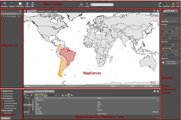
Main Toolbar
Detailed information:Main Toolbar

Here you will find the main tools to customize your workspace. Please bring in Orbit the vector resources provided to you in D:\GENT\ORIGINAL DATA\reference data, only the OVF or SHP files, by drag and drop on the map canvas. Let’s try to see some tools:
- For example save your workspace with the name Gent_workspace, in the same directory and close the software. Reopen it and you will see that your resources are present in the saved workspace.
- With Inspector you can find detailed information about the selected element
- Preferences are user settings, automatically applied and stored for each operating system user independently. Here you can define exactly how Tools in Orbit will perform ( for example you define what parameters of the datasets will be visible in the dataset list, how the zoom will work, how the snap will behave ,the appearance and behavior of the 3D Hover, how you can connect to a database and many more) . For detailed information about each preference setting, see: Preferencesand it’s sublinks.
- All your edits can be saved by pressing Save All
- Select lets you select objects on the Map
- Measure gives acces to measuring tools for the map canvas : lines, circles, angles. Deatiled information on 2D measurements: Map 2D Measurements
Please try to make some measurements on the map to get familiarized. Example :
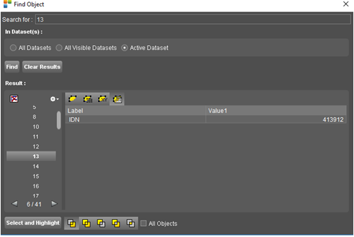
- The search window allows you to search objects in all visible datasets based on an attribute query . For example I have searched for the pole number 13.
- Tools, will be explained later
- Lybrary allows you to add in orbit any supported resource
- The Help icon is important especially for one information, the log file. If you go to Via Orbit interface :
![]() Main Toolbar > Help > About > Details > Open Logfile
Main Toolbar > Help > About > Details > Open Logfile
You will be able to see all actions performed during the last Orbit session. This will help you understand the cause of a certain error or to send this file to Orbit Support Team for further investigation.
Map Canvas
Detailed information: MapCanvas
The MapCanvas is the center of Orbit to view and interact with all your resources. The Orbit desktop has three map views : Map 2D, Map 3D and the Map Layout view. You should take care when swiching between 2D and 3D, the display of resources is different. For example you will not be able to display the Open Street Map in 3D.
On the link above you can find detailed information about each tool, so here we will only concentrate on few ones :
• Navigation gives you extensive choices on how to navigate on the map. Interesting is the function “Move TO” that gives you the possibility to zoom at a desired set of coordiantes, in different CRS
Please try to move to a position at the beginning of your curbstone vector

• Selection, gives you variate possibilities to select objects, including a complex way of querying the attributes tables of your datasets.

Please to Query one of the datasets for specific objects based on their attributes.
• Status Bar, at the bottom of the Map canvas offers some quick, interesting tools :

Here by simply clicking on information you can change it on the fly. For example, if I click on the CRS, I can immediately change the coordinate system of the display. The same for the map scale or coordinates.
Datasets & Dataset Lists
Detailed information: Datasets & Dataset Lists
On the Left side of your screen you can find the Dataset List, that comprises all opened datasets in the list. This datasets can be Runs, vector files, themes, DB, raster files or other kinds of resources.
Open, Import, Create and Remove Datasets
On the upper part from the “+” button you can open datasets, create new ones and more.
As an exercise, please create a new line dataset. This can be done from the dataset list. For detailed information about creating new datasets see: Create New Vector Dataset

Save the dataset in the Gent folder.
Dataset Operations and Indicators in DataSet List
As you can see in your dataset list, around the datasets there are several indicators, each with their role and importance

For example the greyed dataset is the active dataset, the first checked box means that those layers are visible on the map or the last indicator tells if a resource is the recordable one.
But for a compressive explanation of each indicator please read : Dataset Operations and Indicators in DataSet List
As an exercise, please make only the Panoramas, and the poles visible on the map; with the poles the recordable dataset. Your results should be similar to:

Dataset Context Menu
Detailed information: Dataset Context Menu
For each dataset, a context menu is available, which give us access to important information. There are many possibilities and tools in the context menu, we will review the most important next. For the rest please read the information in the link above
• The dataset properties – depicts the general information about the dataset
Detailed information: Dataset Properties Inspect

As you can see, you have the file extension, the type, the CRS the scale for display. Pay attention, if you want to re project a file this isn’t the option for you. Here you can change the CRS if it isn’t assigned at all, or if it was wrongly assigned.
• The dataset structure
Detailed information: Dataset Structure
On the left side we find informations about dataset structure, how many attributes set it has, how many attributes, what kind and more.
For the selected record in the left, on the right part we find detailed information. For example here is the place where you can add new attributes to your file, change the name of the attributes or base them on rules, valuelists, or no rules As an exercise, please open the structure tab for the “measurements” ovf and add another attribute called “Type” based on a rule – ObjectLenght. From now on, any object we draw in this dataset will have this new attribute, and because it is based on a formula, it will be automatically completed with the length of the object.

• Attribute table Detailed information: Dataset Attribute Table View
The “Attribute Table View” displays the attribute component of the active dataset. The attribute values of all dataset objects can be viewed and exported separately for each dataset model and attribute set. An attribute set is one table, the attributes are table columns and one attribute value is one table record. You can sort the attribute table, you can select records or export some records. For example let’s take our “poles” ovf file, open it’s attribute table, linked with the map and select some elements on the map. The records will be selected in the tab too, and ready for let’s say export.
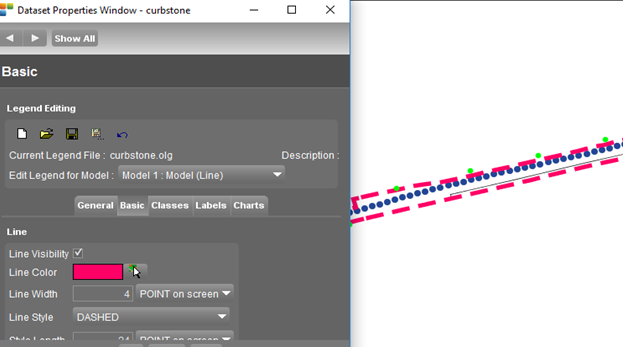
• Legend Editor Detailed information: Dataset Legend Editor
One dataset has one legend file, but each dataset model has its own legend component to be set separately. The legend component depends on the spatial object type (points lines or areas). Spatial resources (vector, raster, image) do not include legend or layout information. Orbit stores the “layout component” in a separated Orbit Legend File (*.olg).
By default Orbit will search and use automatically the .olg file in the same folder and having the same name as the spatial resource file. We do advise this default naming, but this is not mandatory. For example it can be useful to have different presentations for one dataset.
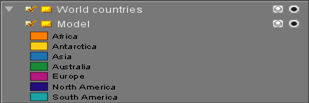
At rhe basic level, we can change the appearance of our resources. For example, let’s make our “”curbstones” more prominent and red . Don’t forget to save the legend if you want it to be kept for future sessions.
But sometimes it is necessary to distinguish objects in the same dataset based on their attributes. Let’s say we want the left curbstone to have one colour and the right another one. In this case we have to edit the information in the tab “Classes”, similar to :
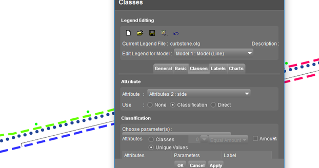
As you can see, based on different attributes, we have different legend styles. This can be applied for any kind of attribute that your data might have.
Please try to create the attribute “TYPE” for curbstones ovf, fill in a value “left” and a value “right” for only two objects ( with the help of Object Inspector, see: Object Inspector) , and create a legend based on this attribute.
• Coordinate reference System
Detailed information: Coordinate Reference Systems in Orbit
Sometimes we have a resource that has an undefined CRS, or we want to convert it to another CRS. From the context menu we have 3 options:
Define Dataset CRS Declare / set / specify the dataset CRS. This will not convert the Dataset CRS. Convert Dataset CRS Transfrom and Reproject the spatial component of the selected dataset. Convert Dataset to MapCanavs CRS Transfrom and Reproject the spatial component of the selected dataset to the current MapCanvas CRS.
Pay attention:
- In orbit for a resource to be correctly displayed on the map it doesn’t need to be in the same coordinate system. As long the coordinates are correct, it is re projected on the fly and displayed on the map in the right position.
- Define Dataset CRS: if the CRS of one resource is “Undefined”, it will be impossible to display; it can also be used only if the dataset CRS is incorrect and you need to define the correct one
Convert Dataset CRS : it will convert the coordinates to another CRS, the position of the resource is displayed correctly in the same place, even if now it has a different CRS
Please exercise and change the CRS for one of the vector layers in our dataset list. Please note that Orbit is basing it’s search of CRS on EPSG codes.
• Save and Export Datasets
Detailed information:
Sometimes it is necessary to save or export our datasets. The difference is that in the first case we only save the dataset with a different name, while in the second we can chose a different export format. So from the context menu of “Panoramas” let’s export them as a .kml file.
Sidebar
The sidebar is located in the right part of the interface and it groups the Tools and Extensions .
Map 2D Tools
Detailed information: Tools Overview
The Map 2D Tools Sidebar provides access to all Orbit's standard tools for spatial editing, constructions, annotations and others like image and raster processing.
It contains 4 tabs with tools combined by their use. It ca be accessed via:
![]() Main Toolbar > Tools
Main Toolbar > Tools
• Edit Tools
In this tab you will find all necessary tools that help you create and edit 2D data
Detailed information :
Create & Edit Objects Overview
You can find all annotation tools in:
![]() Map 2D > Tools > Edit
Map 2D > Tools > Edit
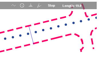
So let’s see what we can do on our data using these tools. For example we want to create new objects. With our “curbstones” dataset active and recordable, we simply draw new objects using the option “New object”
Example, we have added new objects ,continued the streets:
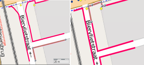
Maybe we are not satisfied with our geometry, then we can add, delete or move some vertexes like in the right image.
And there are many, many tools you can use to: create parallels, split vectors, merge them, rescale objects, rotate them and much more. All of them are explained in detail in the second link of the subchapter.
Please fell free to play with the datasets in our list and edit their objects. Don’t forget to save your modifications if you want to keep them.
• Annotations Tools
Detailed information :
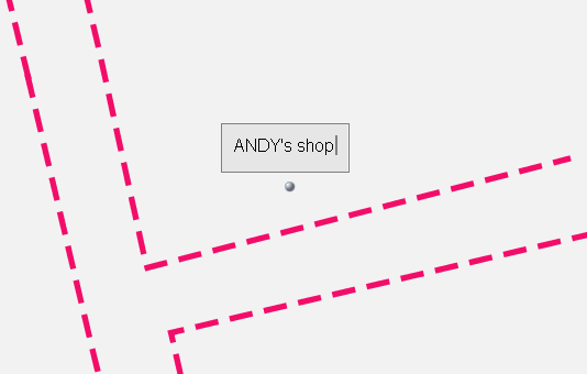
Annotations are tools to complement the map data with temporary notes or sketches. Orbit provides a range of annotation types that can be stored in an annotation file or as attribute (only in OVF format). Since Orbit annotations are georeferenced, they remember exact positions and can be exchanged with colleges.
You can find all annotation tools in:
![]() Map 2D > Tools > Anno
Map 2D > Tools > Anno
So, just create a new annotation file, and start inserting annotations. Several types and forms exists, so are possibilities to edit already created annotations.
• Constructions Tools
Detailed information:
Constructions Overview Construction Tools Sidebar
You can find all annotation tools in:
![]() Map 2D > Tools > Cons
Map 2D > Tools > Cons
Construction tools are used to help you calculate and position exact locations. Look at them as your ruler and measure equipment to set out new coordinates.
There are 2 types of construction tools : Points and Lines. A Construction Point has a single location. You can create as many as you need. A Construction Line as a position and orientation but has no length. You can create as many as you need. Constructions are georeferenced and can be saved in a special file (*.ocf) so you can use them again or forward them to a college.
Construction tools are mostly used to edit objects. While editing objects, the snap function will use constructions as anchor points. For example :
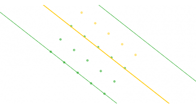
Construction points and lines for drawing road edged perfectly aligned.
There are a lot of possibilities , you can draw constructions based on coordinates, based on paralel or perpendicular lines , bisectrice constructions, parallels based on distances and many more.
• Other Tools
You can find all aditional tools in:
Convert Imagery / Optimize Imagery
Datalied informations:
The “Convert Imagery” tool converts any supported image file into another image file, one on one. Just choose the source file, the target and the format. Of course you can choose the quality parameters.
Please try and export your jpg images as .omi like:
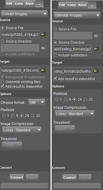 On the other hand, the ”Optimize Imagery” tool converts one or more supported image files into a single Orbit Multiresolution Image. The required information are similar.
Convert Vector Data / Optimize Vector Data
Detailed information:
The ”Optimize Vector Data” tool converts one or more supported vector files into a single Orbit Vector File Tiled. By contrast “Convert Vector Data” tool converts any supported vector file into another vector file, one on one.
Just define the imput, the output,the format or the the CRS and convert.
Please try to convert one of your datasets to a .shp file
Convert Pointcloud Data / Optimize Pointcloud Data
Detailed information:
The ”Optimize Point Cloud” tool converts one or more supported LiDAR files into a single Orbit Point Cloud (*.opc) file. The “Convert Point Cloud” tool converts any supported LiDAR file into another LiDAR file, one on one.
Please try to convert our .opc file to .laz for example.
Merge Datasets / Split Datasets
Detailed information:
http://www.orbitgt.com/kb/orbit_desktop/tools/additional/merge
http://www.orbitgt.com/kb/orbit_desktop/tools/additional/split
Simply merge or split two DataSets. There are two options : you can choose if your models will be merged or added and take care, the legend of the second dataset will be retained. The splitting can be only for the model or for model and tables both.
Create Buffer
Detailed information: http://www.orbitgt.com/kb/orbit_desktop/tools/additional/buffer
A buffer is one or more calculated contours or perimeters around a well defined set of objects or around a fence. The buffer result can be added as annotation, fence or vector dataset or it can be used as reference to select vector data.
The creation is based on a wizard, so let’s try it, and create a buffer around a manhole point. Start by selecting one object, then open the tool.
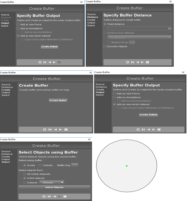
Along the wizard there are many more other optio,ns, like: creating a fence for the buffered objects, create multiplr dimmension buffers or saving the buffer as an anotation.
Georeference image/vector
Detailed information:
Everyone knows georeferencing, is probably the most basic and widely used GIS procedure. It is based on the concept that by knowing the coordinates of certain points we can measure and deduce the coordinates of others.
Before starting georeferencing drag one or several georeferenced layers into the map view. It is important to use all the georeferenced available data to achieve a reasonable result. This is the data that will be used to search control points.
The more detailed and the more recent the information on this data the better the result will be.
• To georeference vector data choose Additional Tool –> Georeference Vector Data
• To georeference image data choose Additional Tool –> Georeference Image Data
We will not exercise it here, being a basic GIS function, but on the link above you can find detailed all the steps. Just as an idea, you have to search for a location in one of both views of which you are able to define the exact same location in the other view. Click in the measure-button in the reference column and point out this specific location in the georeferenced context. The same location will be pointed out with the measure-button in the new image column. When you found at least 3 of such location you are be able to georeference the image. A new textfile with the georeference details will be made and saved under the same path as the location of the georeferenced image.
Make Legend Display Image
Detailed informations:
The “Make Legend Display Image” tool creates an image file from an Orbit dataset legend as it visible in the dataset list dataset legend display.
Browse for the Orbit dataset legend file (.olg), select the required export image format from the drop-down list and enter the size factor to multiply the exported image resolution. The requested image will be created in the same folder and with the same name as the selected olg file.
Spatial Join
Detailed information:
A type of join operation in which fields from one layer's attribute table are appended to another layer's attribute table based on the relative locations of the features in the two layers. A Spatial join is a GIS operation that affixes data from one feature layer’s attribute table to another from a spatial perspective.
You need to define the source dataset, the join dataset (and the attributes you want to join) and the target dataset. As simple as this . Some options for the new objects:attributes are available.
Make 3D Tools
As you can see, if we turn our map in the 3D mode the available tools change to. For this tutorial we are interested in the Point Cloud Tools. ( for example the additional tools were explained on the 2D Tools chapter)
Point Cloud Tools
Detailed information:
The “Pointcloud” sidebar makes it possible to perform and manage point cloud selection. The Point Cloud Selection tools require an Orbit Point Cloud file of the 3rd generation, created from Orbit version 11.0. Tools and buttons of this sidebar will be enabled if the active dataset meets these requirements.
An Orbit Point Cloud file(*.opc) can be used as source file for point cloud selection. A point cloud selection will be saved as Orbit Point Cloud Selection (*.ops). A Point Cloud Selection can be exported to any supported point cloud format or deleted. Deleted points are temporarily stored in the Orbit Point Cloud Deleting file (*.opd) next to the source opc file.
So, we choose a new file, a new selection in fact ( other options are available and explained on the KB link…. to add a selection to a file, to substract from a saved file and more) and we choose “Select”.
We focus on an object we want to select and extract, preferably with top view on. Simply select the object with an rectangle, circle or other option. For example we selected a car:

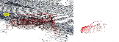
What can we do with this selection? For example we can delete it… this is useful if you want to clean your pointcloud of ghosts, moving objects like cars. Or we can delete just the ground level beneath our object and export a nice, clean object. Like this you can export buildings, entire parts of your run to any supported format.
Please try to export one object from our run.