Content Manager Tutorial

This tutorial explains the typical workflow to use in Orbit MM Content Manager. It will guide you through the steps required to process and organize mobile mapping data, but for detailed explanation of each tool it is necessary to read the information on the Knowledge Database: http://www.orbitgt.com/kb/

Software : Orbit MM 11.2.3

Software homepage: Orbit Mobile Mapping Content Manager

Data : Generic , Gent, Belgium. Input data: Panoramic images (jpg), photo positions (csv), lidar data (las), ground control points (txt). Please copy the demo data provided to : D:\training\GENT

Necessary knowledge: Before starting working with the CM it is advised to first understand how Orbit sees MM data and what kind of data can be used. For this please read:

• Understand Mobile Mapping data in Orbit
• Supported Resources for Mobile Mapping

Detailed explanation: Orbit Desktop Installation

The first step is to install the software. This requires to register on orbit’s website and download the desktop product.

Installation is simple, it requires just to click the executable and a folder will be created by default in: C:\Program Files\, called Orbit GT containing separate folders for each Orbit product. Also, a desktop shortcut will be created, and by opening it, you will be prompted to enter your activation key. If you didn’t already received one, you can submit a request and you will receive it.

This requires outbound internet connectivity, for more details read: Orbit Online License Activation

Sample data used in this tutorial can be downloaded from :

Detailed explanation: MM Data Preparation and Import Templates

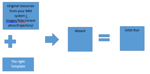
You can bring your mobile data into Orbit by using Templates. An Orbit import template is a predefined set of configurations, containing all technical details of the mobile mapping system. A template is exactly configured according a given vehicle setup, used sensors and available resources. This technique simplifies and standardizes the workflow to import a well known set of mobile mapping resources.

On the above KB page you will file a list of available templates for download. After the download the template must be unzipped and copied to the Orbit installation folder : <Orbit installation directory>client/program/ext/mobile_mapping/project/template/

There are two kind of templates: generic templates and vendor adapted templates, for each type, in the above KB page you will find in the table a link to a page that describes exactly how the data should look, called “Prepare MM Data…..”

The generic templates are designed to be used for data exported from any mobile mapping system with minimum customization. You have available for download generic templates for only Lidar data or only imagery or both, and different templates if you use data in a geographic coordinate system or in a projected CRS. Be careful , your data format must match exactly the formats explained in detail in : Prepare MM data Generic Import

In the vendor adapted section of the table you will find templates for the main systems on the market. You can download the appropriate one for you and read in the “”Prepare MM Data….” How the data should look. For example, for data exported from a Leica system, you should read: Prepare MM Data Leica

Templates can be also adjusted to suite your data, but this requires more knowledge, or new templates can be created by the Orbit Support team.

In our training scenario, we will use the Generic_ LiDAR Pano template provided in the sample data, so please copy it to the Orbit installation location mentioned above.

Detailed explanation: Import Mobile Mapping data in Orbit

The next step is to import your data into Orbit, and the procedure can be summarize like this :

To start the import procedure, go to:
Procedures > Administration > Mobile Mapping > Import Run

The import is based on two wizards, and by following the steps in them ( explained in detail on the Kb page mentioned above) you wull be able to bring all your data into an Orbit structure.

The first wizard creates the run definition, you must choose a unique name for your run, the template you want to use and a destination folder where your data will be stored.

In our training, we can use the following:

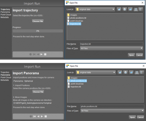
The second wizard is dedicated to importing your resources. Based on the template chosen, the following items might be imported:

• Trajectory – choose the trajectory file
• Panorama – choose the photo positions file and move images to the directory shown in the wizard
• Pointcloud – choose the lidar file
• Metadata – complete some information, optional

In our case, we will choose:

Don’t forget to move jpg images from D:\GENT\ORIGINAL DATA\original data\images, to the exact folder mentioned in the capture above.

After all steps are done, press finish.

If the import is successful, the imported resources will be displayed in the dataset list, and the photo positions on the map. To see the resulting run folder structure and files you can go via Windows to the location where you saved the run, in our case: D:\GENT\gent_training

Detailed explanation: Manage your Mobile Mapping Runs

We have our data imported, but there are other operations that can be applied to runs in Orbit :

• Open Run – if you have already imported a run you can open it anytime with this procedure

• Add Run - if you have removed a run you can add it again

• Edit Run – you can edit a run ,by changing only one resource; for example you added on import the wrong pointcloud file. By simply choosing a new pointcloud file, your run will be updated

• Remove Run – if you think that you don’t need a run any more , you can simply remove it. The data will not be erased, only the run will no longer appear in the list of available runs.

All this can be started from :
Procedure > Administration > Mobile Mapping >

All are based on very simple and intuitive wizards. Please try to play with the run created before and remove it, add it again or edit one of the resources to see what happens.

Also from the same location, there are other options available :

• Process imagery
Detailed information: Process MM Imagery
You can work in orbit with any forma of supported images, but for better performance, especially for publishing MM data, it is advised to process your imagery into an orbit native format.

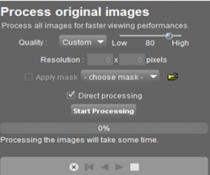
In our case we will process the .jpg images into .omi – Orbit Multiresolution Images.

Again it is a simple wizard, you just have to set the quality of your .omi result or the resolution. It makes no sense to process at higher quality then the input images. Usually, an 80% quality is more than enough. In our case:

It takes some time to process imagery, so if you have a huge number you can disable the Direct processing and process with Task manager over night for example.

The results will be found in : D:\GENT\gent_training\panorama1\processed

• Process Point Cloud Image
Detailed information: Process Point Cloud Image

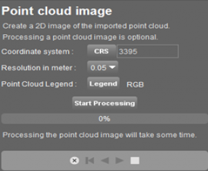
This procedure allows you to create a 2D ortophoto from the pointcloud, topview. It is useful for digitization or if you don’t have a reference map .

Again it uses a simple wizard where you can set the CRS, the resolution and the legend of the pointcloud. In our case:

The result will be added to the dataset list.

Detailed information: Manage your Mobile Mapping Projects

Sometimes, you have a huge volume of data, multiple runs. It might be necessary to group this runs in a logical manner, and this logical way is by projects.

A project is a list of mobile mapping Runs, a logical grouping without data duplication, for which permissions can be set. All included Runs must have similar structure of resources and coordinate system.

Projects don’t contain the physical data, they are only pointers to a list of Runs known by Orbit. Runs can belong to multiple projects. If Runs are imported correctly, there are no limitation on volume nor size of Projects. Theoretically there is no limitation on the number of Runs combined by one Project. So, is your decision what runs you will include in a project. For exampleyou can group by geographical area, mapping project, date or year. The main advantage is that all your runs will be displayed together on the map.

The operations applicable to projects are similar with the ones for runs.

•Create Project
Procedures > Administration > Mobile Mapping > Create Project

•Edit Project
Procedures > Administration > Mobile Mapping > Edit Project

•Remove Project
Procedures > Administration > Mobile Mapping > Remove Project

•Open Project
Procedures > Mobile Mapping > Open Project

•Close Project
Procedures > Mobile Mapping > Close Project

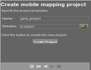
Let’s try now to create a project. We only have one run, so it’s not the best example, but the procedure is the same. Simply initiate the Create Project procedure, choose from the list the runs you want to include in the project. In the next wizard choose the name and location, like this:

The project will be created and loaded. If we would have more runs, all off them will be displayed. In the Gent folder anew folder named gent_project will be created that links the project with the phisical data in the run directory. Please try the other options availabe, to edit, close or open a project. The action is similar as for runs.

Now, that we have our data imported, we will want to open some MM Views in order to navigate through the data, check it or make measurements.

Detailed information:Open Mobile Mapping View from Map

To achieve this we have to go to:

Tabs > Mobile Mapping > Top Toolbar > Open View

The “Open View” function, operated by the left mouse button, makes it possible to open one ore more mobile mapping views by indicating a position on the Map. The active “Open View” function is indicated as “Place Point” in the map status bar and the appearance of the mouse pointer as “Cross” when hovering above the map. A newly opened view is always opened with a field of view equal to 90 degrees.

There are several ways of opening a view, described in detail in the KB page accessible by the link above.

To close a single mobile mapping view hover above and click on its reference number in the mobile mapping view sidebar. Close all views via the according “Close all” button in the mobile mapping view top toolbar.

Please try to open views on our run using the described ways.

Detailed information: Navigate on mobile mapping image view

By accessing the link above you will find a description of each type of mouse click action and the resulting navigational behavior.

Please try to accommodate yourself with navigating on MM views.

Detailed information: Navigate in mobile mapping 3D point cloud view

By accessing the link above you will find a description of each type of mouse click action and the resulting navigational behavior. Please note that to navigate through the 3D point cloud some mouse actions are different than the ones used to navigate on MM views.

Please try to accommodate yourself with navigating on 3D point cloud view.

Detailed information: Mobile Mapping Top and Side Toolbar

Let’s see next what options we have to customize the display on MM views.

All tools are grouped on the left side and top of the view, in two tollbars. Please see the detailed description of each icon by accessing the link above. Pay particular attention to the ways you can change the presentation of the pointcloud, detailed informations here: Point Cloud View and Restriction Settings on Mobile Mapping Views

Try to play with each function in order to get familiarized with them.

Detailed information: Measurements on Mobile Mapping Views

One of the most important functionalities of orbit software is the ability of making measurements directly on MM images and pointcloud. So, next we will see how we can measure and what types of measurements we can do.

To start measuring go to :

Tabs > Mobile Mapping > Opened View > 1st View Side Toolbar > Measure icon

The following window will appear:

As you can see there are a lot of measure functions. For a detailed explanation of each one please see: Map 3D Measurements

There are two modes to measure : using pointcloud or measure using triangulation. You can choose the mode by enabling or not the “Use point cloud” option.

A point cloud resources must be available for at least one of the currently opened views to enable the option “Use point cloud”. If there is no point cloud resource available for any of the opened views, this checkbox will be disabled. In case the option is enabled and a measurement using point cloud is done within a view without point cloud the message “No point cloud available for this image.” will be shown.

In theory, measurements using the pointcloud are more exact. You don’t need to have the pointcloud visible on the view to measure based on it; as long the option “use point cloud” is enabled the point cloud is behind and measurements will be based on lidar points spatial position.

For detailed information about measuring using the pointcloud see: Measurements with a single click using Point Cloud

For example, let’s measure a distance on one MM view in our run. Your result should look similar to:

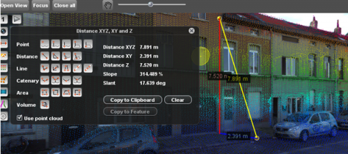
Please try to measure some points, distances, lines, areas or volumes on our run.

For detailed information about measuring using triangulation see: Measurements via triangulation using 2 images

The same measurement using triangulation.

Please try to measure some points, distances, lines, areas or volumes on our run using triangulation.

Another important topic on measurements is about the 3D Hover. See detailed information about the 3D hover on: Preferences of 3D Hover

The 3D Hover (“yellow puck”) represents the on the fly detected 3D surface around the position of the mouse pointer. The hover is based on screen pixels within the given query “Search Radius” for which a coordinate is known. A pixel coordinate can be derived from any visible dataset object from point cloud, vector or image resources. Overlays are not taken into account. If, given the 3D Hover Query settings, no 3D surface can be detected around the mouse pointer position as seen from the current 3D view point, no hover will be displayed no 3d coordinate measurement will be possible.

There are 3 measure technique to be used for measurements. You can choose the technique from the 3D Hover preferences:

Main Toolbar > Preferences > 3D Hover

• Closest Point - the coordinates of the closest lidar point will be the coordinates of our measurement

• Flat Surface Intersection (default) – the hover will try to detect a flat surface intersection and this coordinate will be taken into account

• Ridges and Corners Intersection- it will try to detect where a ridge or a corner is located and take it’s coordinates as base for our measurement

You can chose the proper technique for a measurement based on the object you are trying to measure and on pointcloud density.

For example, on a dense pointcloud junction between the street and the sidewalk is best measured using the ridge detection or the flat surface intersection. Or, in the same dense pointcloud, a point representing a manhole can be easily measured using the closest point. The same manhole , in a sparse pointcloud will be measured using flat surface intersection, because the closest point might be far from the actual position… and so the error big.

The final topic on measurements is about saving your measurements. A measurement is only that, the area you drawn for example will disappear as soon you start another measurements. But sometimes we need to keep all measurements as objects or to at least keep the results.

For this in the Measurements Window above you can observe two important options :

• Copy to clipboard: will copy the results of your measurements to clipboard , from where you can paste them in a document for example. For example bellow the copied results of our last measurement

Distance XYZ Distance XY Distance Z Slope Slant Error 8.037 3.160 7.390 233.858 23.152 0.008

• Copy to feature: the measurement will be copied as a vector object in a dataset. A dataset of the same type must be available in the dataset list ( point, line, area), it must be the selected dataset and must be recordable.

As an exercise, please create a new line dataset. This can be done from the dataset list

For detailed information about creating new datasets see: Create New Vector Dataset

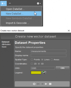
Save the dataset in the Gent folder, and make it recordable. For detailed information regarding datasets& dataset list see: Dataset Operations and Indicators in DataSet List

Finally, press “Copy to feature” and your measurement will be saved in this dataset.

Detailed information: Vector Overlays on Mobile Mapping Views

You might have some vector resources from the area of your MM run, from external sources or from your measurements, that you want to see in your MM view.

Any 2D or 3D supported vector resource can be overlayed on mobile mapping images or 3D point cloud view. Images and raster resources cannot be overlayed. To overlay a dataset special attention is required to the dataset coordinate reference system, structure definition and legend.

For this there are two options:

Dataset List > Dataset Context Menu > Display in Mobile Mapping

Dataset List > Dataset Indicators > Extension Indicator

You can set the preferences of the overlays from the MM view sidebar.

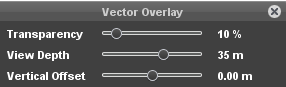
Pay special attention to the vertical offset. To display a 2D dataset in a 3D environment, a reference ground Z value is calculated for each 2D object vertex. The vector overlay vertical offset is only applied on 2D objects. The height (Z coordinate) of 3D objects will be respected as is. If a 2D datset is set incorrectly as a 3D structure, the Z value (=0) will be respected as is. Most probably these objects will not be visible because of displayed far below reference ground level of the 3D mobile mapping resources.

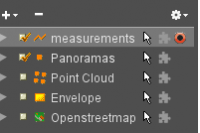
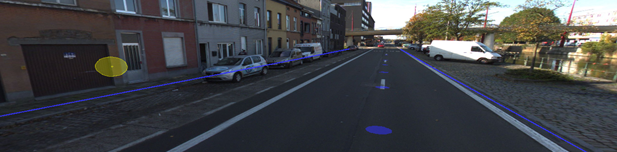
In our case, in the sample data we have (D:\GENT\ORIGINAL DATA\reference data) several vector files.Take for example the “curbstone.ovf” file and simply drag and drop it on the map. Make it visible :

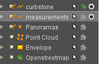
Now, you should see the vectors displayed on the MM view:

Extensions are tools especially designed for a particular software module, in our case the Contant Manager. You wuill not find these tools in other modules.

They can be reached by :

Main Toolbar > Extensions

Detailed information:Mobile Mapping Catalog

The mobile mapping “Catalog” extension gives a complete overview and detailed information of all mobile mapping runs and projects. The interactive combination of map (geographical information), table (overview) and sidebar (detailed information) result in a powerful mobile mapping management tool.

It can be accessed via: Main Toolbar > Extensions > Catalog

From the sidebar view tab, you can select on the Map the run you are interested, in order to view it’s details or you can remove or archive the selected run. There are different options to display runs or projects, to color them differently. Important also is the option to display the trajectory. By checking it, the trajectory information will be displayed on the map, including different coloring by GPS accuracy.

Your display should look like:

In the sidebar Inspect tab you will find detailed information about the selected run.

Please familiarize yourself with the options and also enable the trajectory, because we will need it later in our exercises. Your display should look like:

Another way of viewing your data and information about it is from the Catalog Tab. Here you will find the complet list of you MM runs and projects. Again you can archive for example some runs you don’t need anymore. This will not delete the physical data.

If information about your run is missing ( number of images, size on disk ) please use the context menu and the option Recalculate Data Volume.

Detailed information:

Mobile Mapping Ground Control Points

Ground control points are points measured on the ground in a ground survey. Their position is known, with an accuracy of millimeters or a few centimeters.

We can use such points to adjust our data. By remeasuring them on the MM views, we can find the differences between our data and the ground survey and in the next step to adjust our data.

Using ground control points (gcp's) one can verify the absolute accuracy of the mobile mapping data by measuring the position of exactly known reference points within a given time period subset of mobile mapping data. Measured ground control points can be used by the ”Trajectory Adjustment” extension to correct the absolute position of trajectory, image positions and point cloud data.

On import gcp's are linked to the trajectory by time-stamp based on their geographical proximity. If multiple distinguishable trajectory segments are within the critcal distance to the gcp, the gcp will be linked to each occuring trajectory time stamp.

This extension can be accessed via :

Main Toolbar > Extensions > Control Points

As you can see in the sidebar the first step is to add a file with GCPs. It can be an orbit vector file, a shapefile. We can also use a simple TXT file (with columns corresponding to gcp number , x,y,z) that we drag and drop into Orbit and then export it as a vector file. See export dataset:

http://www.orbitgt.com/kb/orbit_desktop/export/exportdataset/exportdatasetto

In our case we will use an ovf file ( found In : D:\GENT\ORIGINAL DATA\ground control points); Please add the gcp_4326_touse.ovf. As you can see, the GCPs will be displayed on map and as a list in the sidebar.

The next step is to measure them. For this, open one MM view and simply double click on one point in the sidebar list. This will focus the view on the desired point ( let’s take the first). Navigate through the view in order to have a good viewing angle of the point – pay attention, it might be under the car, so go to next image to see it.

When the point is focused, simply click measure and place the point in the right location. Normally you will have from your surveyor some photos of the location of the point in the field. In our case it is known that the points represent the center of the manhole. Your measurement should look like this:

In order to get more accurate measurements pay attention to the 3D hover preferences explained earlier.

Procede and measure the other four points in the list. Your results shouls be close to :

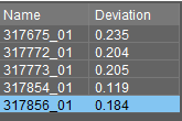
You can clear a measurement and re do it or you can remove a point from the list. You can choose to display all GCPs or onlythe ones outside tolerance. From the slider you can adjust the tolerance value according to your project requirements. The areas where more GCPs are falling outside the tolerance will need to be adjusted.

Detailed information: Mobile Mapping Trajectory

Now we have our measured GCP’s , the next step is to adjust the trajectory.

Sometimes, due especially to GPS signal accuracy it is necessary to adjust your data. As you can see in the screenshot above, there are areas (in blueish color) where the accuracy is not very good. Because trajectory is linked with images and pointcloud by timestamps, it is possible to adjust the trajectory and in this way to adjust the data.

The adjustment is based on ground control points that we have from a ground survey. A well defined segment of a run can be adjusted or removed. An adjustment is calculated using all available measured ground control points. Removing or adjusting segments will affect all resources.

The extension can be accessed via :

Main Toolbar > Extensions > Trajectory

So let’s try to adjust our trajectory:

• First, create a new segment and select it either on the map or on the graph

• We will adjust the segment where our GCP are located , which is also the segment with low accuracy. Your selection should be similar to:

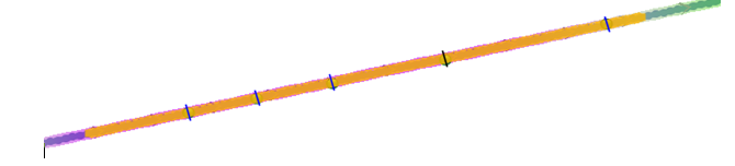
1 in orange the selected segment

The selected portion of the trajectory will be displayed in the Trajectory graph also, or the selection can be made in here.

The vertical lines represent our measured GCPs in blue and in black the selected one.

On adjusting a segment using the trajectory adjustment extension the relevant snapshot of the ground control points dataset will be saved and used for future processing. Any measured ground control point within 10 meter (xyz) to the trajectory segment will be retained.

A quick preview of the adjustment for the opened segment only can be pre-processed. This will not correct or remove data of the run. All corrections (adjustments, remove segments and remove point cloud points) will be applied on the next step – Consolidation.

So, enable the Process preview icon and press Adjust. Remember this is just a preview on how the data will look if we will consolidate our adjustment. To see the results, check “Show adjusted Data “ and open a MM view on the location of a GCP. You shouls see the following result for the first GCP :

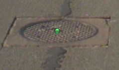
As you can see, the GCPis now at the right location, so the images and the pointcloud were correctly adjusted.

There is also the option of removing a segment that we don’t need , for example a segment in a multi-pass area. The procedure is similar, just press “Remove” instead of “Process”.

The adjustment is linear, which means that is strongest around our GCPs and fades out linearly at the end of the segments. The effect of the adjustment can be prolonged till the end of the trajectory or from the beginning with the options “adjustment in or out “.

Detailed information: Mobile Mapping Consolidation

We have calculated the necessary adjustments, seen on the preview thet the adjustments are proper, if we want to aply the adjustment to the data, we have to use this extension, which can be reached from:

Main Toolbar > Extensions > Consolidation

The mobile mapping “Consolidation” extension applies all corrections as defined via the ”Trajectory Adjustment” extension and 3D point cloud cleaning tools. A single source run will be consolidated in a new 'cleaned' target run.

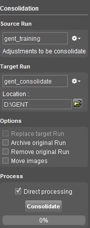
All we have to do is to define the source Run, the target Run and it’s location and press “Consolidate”.

The result will be a new run, containing all the resources from the source, but adjusted. You can find and verify the results in: D:\GENT\gent_consolidate

There are available options to archive, or remove the original run.

Detailed information: Mobile Mapping Delivery

The “Delivery” extension makes it possible to export a selection of mobile mapping data in several output formats. This can be either in Orbit structure or a generic file-format, and you can export only one type of resource from a particular run (for example only the pointcloud) or all resources in a run.

It can be accesed from:

Main Toolbar > Extensions > Delivey

Basically we have to choose what we want to export, the name and place of the results and the export format and characteristics.

In our case we will export for example the vectors in .shp format and our pointcloud in las format.

So, we create a new delivery and then chose from the catalog tab our run, add it to the delivery with the option “Add to delivery” from the context menu. You can even draw a fence and export only a part of the run.

The results will be in: D:\GENT\gent_delivery. If you check inside all vector data folders (envelope, trajectory, photo positions) you will find new files in .shp format.

Please repeat the exercise and export the pointcloud in .las format.

Like all time consuming processes (image processing, pointcloud optimization, consolidation) this phase can be performed using the Task manager if you have a big data volume. Just disable “direct processing” and the task will wait for you to start it in task manager at a convenient moment.